
Final Project
PIC 16B Project Group Submission
1. Introduction
We wanted to find out whether or not quarterly earnings conferences give any extra insight into how a company is doing financially compared to the raw data. To this end, we regressed daily price changes with different aspects of earnings reports with linear regression and neural network models, and did a sentiment analysis on earnings conferences to see if either one has any relation, or if one has a stronger relation with future changes in value than the other. Here is a link to our GitHub page for the project.

Flowchart:
2.1 Data Imports and Organization
To build our working dataframe we used the SimFin API to pull the (numeric) financial statements for all available quarterly reports.
# Set your SimFin+ API-key for downloading data.
sf.set_api_key('H9OLpPRQ36sXqfhoOtyBb0Kwv4Dw0q3W')

# Set the local directory where data-files are stored.
# The directory will be created if it does not already exist.
sf.set_data_dir('~/simfin_data/')

# Download the data from the SimFin server and load into a Pandas DataFrame.
quarterly = sf.load_income(variant='quarterly', market='us')

# Print the first rows of the data.
#print(quarterly.head())
quarterly.head()
We then repeated the same procedure to build a company df containing SimFinId, company name, and sector info:
# Download the data from the SimFin server and load into a Pandas DataFrame.
companies = sf.load_companies(market='us')
and then the same for a translational dataframe between industry id and industry name
# Download the data from the SimFin server and load into a Pandas DataFrame.
industries = sf.load_industries()
print(industries["Sector"])
From here, we needed to build a df of stock price data (open/close price, volume, etc.):
# Download the data from the SimFin server and load into a Pandas DataFrame.
shares = sf.load_shareprices(variant='daily', market='us')

# Print the first rows of the data.
print(shares.head())
#print(shares["Date"].head())
print(shares.columns)
print(shares.index)
#so date is a part of a multi index, not a column
#lets reset that index to get these as columns for easier bool syntax
shares = shares.reset_index()
#see if that worked
shares.columns
#lets examine the types for any future comparison issues
print(shares.dtypes)
#okay so its a datetime, need to make sure other dates are in this format
#pd.to_numeric(shares.Date) - incase the other isn't, convert to float
print(shares.head())
We then merged these on the appropriate report release dates for each ticker for each report to create a single, unified, working pandas dataframe, from which we calculated our target variable “DeltaPrice” (the difference between close and next day opening price as a measure of after hours price movement in response to a given quarterly report) and populated a new column with it:
# Combining databases

merge1 = pd.merge(quarterly, companies_tick, how = 'left', on = 'SimFinId')

alldata = pd.merge(merge1, industries, how = 'left', on = 'IndustryId')

print(alldata.head())

#lets see what our types are
Alldata.dtypes
y(lambda row: row["NextDay"] - row["Close"], axis=1)
From here, all that remains data handling wise, is specific to each application going forward (e.g. dropping unneeded columns or encoding for LR)```
shares["NextDay"] = shares["Open"].shift(-1)
#alldata.rename(columns ={'Publish Date': 'Date'}) - figure out why rename isn't recognizing Publish Date

#hacky short term solution
alldata["Date"] = alldata["Publish Date"]

shares2 = shares[["SimFinId", "Open", "Close", "Date", "NextDay"]]
alldata = pd.merge(alldata, shares2, how = "left", on = ["SimFinId", "Date"])
#cool, now we have everything together, I'll clean this up to only be what we need instead of a bulk merge later


alldata["DeltaPrice"] = alldata.appl
2.2 Regression
To start with the numerical analysis, we created a linear regression model, which took in the numerical values from the dataset, and regressed them onto our variable ‘DeltaPrice’, which we created by subtracting the close date from the open date of the next day for each datapoint. We then used sklearn’s LinearRegression model to regress the data, and put all of this, as well as a train-test-split testing mechanism into a function that takes in a subset of our main dataframe to perform the linear regression. With the whole dataset, the linear regression performed at around 31% accuracy, which we considered to be good, since it is predicting the exact change in price, for which there are many values. Below is the code for the function:
def lr(df = newdata):
  mlinx = []
  mliny = []
  regx = df.drop("DeltaPrice", axis = 1)
  for i in df["DeltaPrice"]:
    mliny.append(round(i, 2))
    mlinx.append([])
  for i in regx.columns:
    k = 0
    for j in regx[i]:
      mlinx[k].append(j)
      k += 1

  X2 = sm.add_constant(mlinx)
  est = sm.OLS(mliny, X2)
  est2 = est.fit()
  print(est2.summary())
  j = 1
  for i in regx.columns:
    print(str(j) + ": " + i)
    j += 1
  X_train, X_test, y_train, y_test = train_test_split(mlinx, mliny, test_size = 0.2, random_state = 42)
  LR = LinearRegression().fit(X_train, y_train)
  print("Test score:")
  print(LR.score(X_train, y_train))
  return X_train, y_train
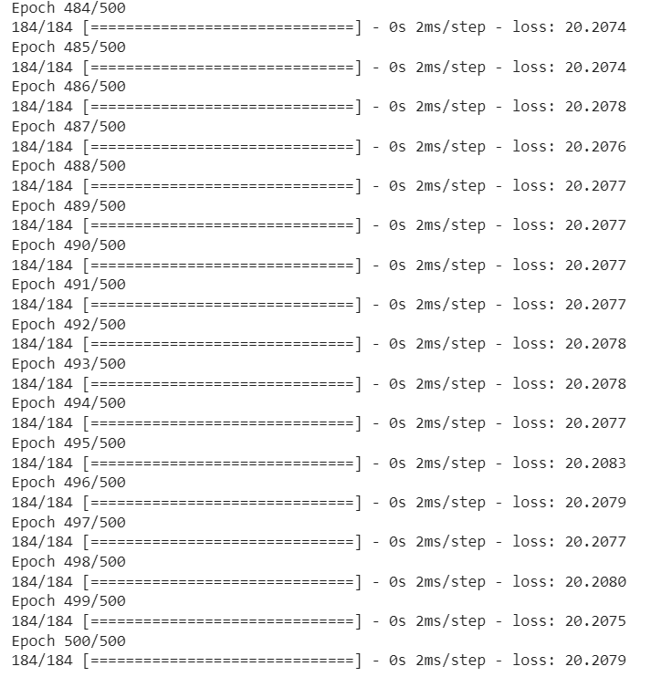
For the neural networks, we used a similar format as for the linear regression model, but we changed it so that the user can input which sector they would like to run the regression on, since the model is too big to run on the whole data, and we got better results from running it on just one sector than on the whole dataset, and whether they would like to use the model with or without the LSTM, or long short term memory, layer. We found that the model works moderately well without the LSTM, but produces meaningless results with the LSTM layer, so the default setting is without the LSTM layer. Below is the code for the function, and a screenshot of some of the last epochs of the model run without LSTM on the sector ‘Healthcare’, which have a loss of around 20.
def nn(sector="Technology", rnn = False):
  rnndf = regdata[regdata["Sector"] == sector]
  rnndf = rnndf.drop(["Sector", "Industry", "Date", "NextDay"], axis = 1)
  rnndf = rnndf[rnndf["Close"] != 0]
  rnndf["PctChg"] = rnndf.apply(lambda row: round(1000 * (row["DeltaPrice"] / row["Close"])) / 10, axis=1)
  rnndf = rnndf[rnndf["PctChg"] < 70]
  rnndf = rnndf[rnndf["PctChg"] > -70]
  rnnx = rnndf.drop(["DeltaPrice", "PctChg"], axis = 1)
  cmp = rnndf["SimFinId"]
  cmp = cmp.drop_duplicates()
  ryl = []
  rny = rnndf.sort_values("NewDate", axis = 0)
  for i in rny["PctChg"]:
    ryl.append(round(i, 2))
  rxl = []
  rnx = rnnx.sort_values("NewDate")
  for i in rnx["NewDate"]:
    rxl.append([])
  for i in rnx.columns:
    k = 0
    for j in rnx[i]:
      rxl[k].append(j)
      k += 1
  rxa = np.array(rxl)
  rya = np.array(ryl)
  if rnn:
    model.fit(rxa, rya, epochs=50, verbose=1)
  else:
    model1.fit(rxa, rya, epochs=500, verbose=1)
2.3 Scraper
To gather transcripts, we used the Financial Modeling Prep API. We first built a function to structure and individual query:
def call_pull(ticker, year, quarter,key = '8dccdfa88c60658c4170dbaa660a6c5c',
             date=False):
   transcript = requests.get(f'https://financialmodelingprep.com/api/v3/earning_call_transcript/{ticker}?quarter={quarter}&year={year}&apikey={key}').json()
   tran = transcript[0]['content']
   date = transcript[0]['date']
   if (date):
     return [tran, date]
   else:
     return tran

Next we build a function to automate the pulls for each entry in a provided data frame:
def transcript_fetch(df):

 df["Fiscal Period"].str.slice(1,1)

 #make transcript column
 df['Transcript'] = ""

 #start a counter
 count = 0

 # for each company ticker
 for ticker in df["Ticker"]:
   #for each call date
   for date in df["Publish Date"][df["Ticker"] == ticker]:
     #get quarter from fiscal period
     for period in (tech_sample["Fiscal Period"][(tech_sample["Ticker"] == ticker) & (tech_sample["Publish Date"] == date)]):
     #pull numeric value only
       quarter = period[1]

     #pull year
     #month = date.month
     year = date.year

     count +=1

     #pull transcript
     try:
       trans = call_pull(ticker, str(year), str(quarter))

       #convert to string
       trans = str(trans[0])

     #if pull fails
     except:
       trans = np.NAN #make NAN for later drop

     #add to "Transcript" column
     tech.loc[((tech["Publish Date"] == date) & (tech["Ticker"] == ticker), 'Transcript')] = trans

 #return df now with transcript strings
 return df
Notably, the Fiscal Period returned by the API is actually a not-too-well-documented object, not a string, and so required an uncomfortable amount of hacky syntax to coax say, the numeric only “1” string out of a Q1 fiscal period OBJ.
2.4 Sentiment Analysis
From here, largely on account of our late-dropping group member, we had to curtail our pulls to random samples (n=1000 and n=2000). However, we did have nice syntax prepared to tokenize and core the text using our sentiment dictionaries and add these elements as new rows to our dataframe:
import pandas as pd
from nltk.tokenize import WordPunctTokenizer as wpt
import nltk

nltk.download("opinion_lexicon")

from nltk.corpus import opinion_lexicon

pos_list=list(opinion_lexicon.positive())
neg_list=list(opinion_lexicon.negative())
print(pos_list)
#for each transcript
for transcript in final_sample["Transcript"]:

 # Tokenize the words and convert to lowercase
 text = transcript.split()
 text = [text.lower() for text in text]

 # Remove the stopwords
 text_clean = [word for word in text if word not in stopwords]

 words_pos = [word for word in text_clean if word in pos_list]
 words_neg = [word for word in text_clean if word in neg_list]

 pos_score = len(words_pos)
 neg_score = len(words_neg)

 tokens = lm.tokenize(transcript)
 score = lm.get_score(tokens)

 final_sample.loc[((final_sample["Transcript"] == transcript), 'Positive')] = pos_score
 final_sample.loc[((final_sample["Transcript"] == transcript), 'Negative')] = neg_score
 final_sample.loc[((final_sample["Transcript"] == transcript), 'Ratio')] = pos_score / neg_score
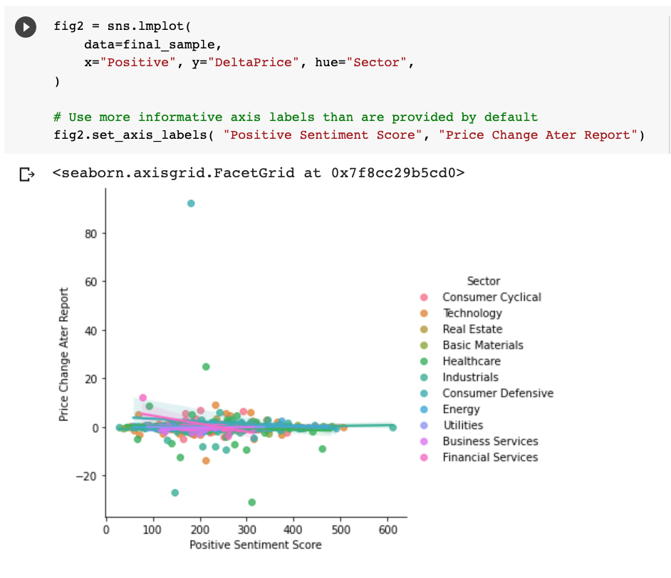
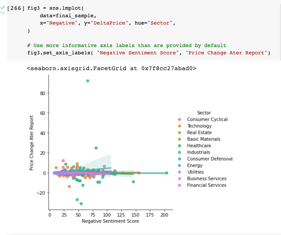
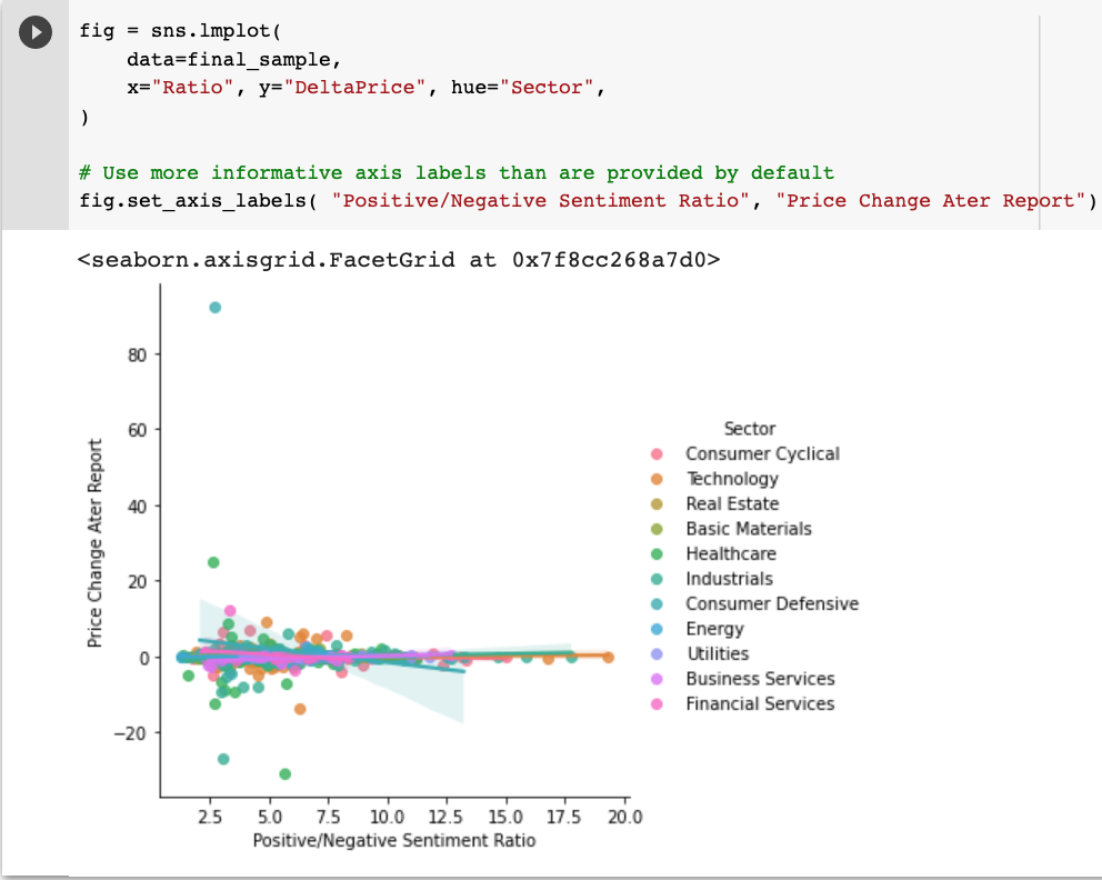
We then used seaborn to plot the relationship between positive, negative, and pos/neg ratio scores and our target variable of DeltaPrice:
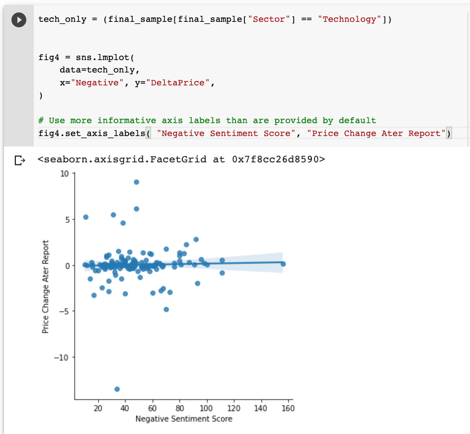
We also plotted the technology sector in isolation and noticed a curious group of points where “no bad news” seemed to be more strongly correlated with DeltaPrice than actual positive sentiment or even the ratio of positive to negative sentiment:
3 Conclusion
We found that recurrent neural networks do not work very well on stock data, and that our linear regression model does surprisingly well. On the sentiment side, the plotted results were very much undermined by the lack of time to run full 36,000+ row pulls. The random samples undermined any patterns found within the time series of a particular company for both the sentiment analysis and the neural networks. Ideally, moving forward we would run a complete S&P 500 pull (to avoid potential noise from small-caps), and precluding reports from the period of extreme Fed Quantitative Easing in response to COVID (or isolating and analyzing them separately). Similarly, we would like to follow through with our original intent to both run a neural network model on vectorized transcript text and to see the effect of the inclusion of sentiment scores as features within our most successful numeric model.