HW4 - Fake News Classifier

Classifying Misinformation with NLP

For this assignment we’re going to develop a misinformation (colloqually “fake news”) classifier using TensorFlow.

Our data for this assignment comes from the following article:

Ahmed H, Traore I, Saad S. (2017) “Detection of Online Fake News Using N-Gram Analysis and Machine Learning Techniques. In: Traore I., Woungang I., Awad A. (eds) Intelligent, Secure, and Dependable Systems in Distributed and Cloud Environments. ISDDC 2017. Lecture Notes in Computer Science, vol 10618. Springer, Cham (pp. 127-138).

And is found by way of Kaggle. Here we’re going to use a pre-split version of this data as graceously provided by UCLA Mathmatics Professor, Phil Chodrow, using the link found below.

train_url = "https://github.com/PhilChodrow/PIC16b/blob/master/datasets/fake_news_train.csv?raw=true"

Now let’s get the slew of imports handled:

#import the usual suspects
import pandas as pd
import numpy as np
import tensorflow as tf

#import string + regular expressions...just in case, don't presume base pkgs...
import re
import string

#import keras, layers, loss functions etc 
#ignore the yellow warning, currently a bug even on colab...a google product
from tensorflow.keras import layers
from tensorflow.keras import losses
from tensorflow import keras

#imports for text handling (vectorization etc.)
from tensorflow.keras.layers.experimental.preprocessing import TextVectorization
from tensorflow.keras.layers.experimental.preprocessing import StringLookup

#for visualizing model layers
from tensorflow.keras import utils

#imports for encoding and our splits, the sklearn classics
from sklearn.preprocessing import LabelEncoder
#used if you prefer to split at the df rather than ds stage
from sklearn.model_selection import train_test_split

# for simple visualizations (line graphs)
from matplotlib import pyplot as plt

# for embedding visualizations
from sklearn.decomposition import PCA
import plotly.express as px 
import plotly.io as pio
pio.templates.default = "plotly_white"

From here let’s read in the data:

#csv read in via pandas
raw_df = pd.read_csv(train_url)

Let’s take a look at what we have:

raw_df

	Unnamed: 0	title	text	fake
0	17366	Merkel: Strong result for Austria's FPO 'big c...	German Chancellor Angela Merkel said on Monday...	0
1	5634	Trump says Pence will lead voter fraud panel	WEST PALM BEACH, Fla.President Donald Trump sa...	0
2	17487	JUST IN: SUSPECTED LEAKER and “Close Confidant...	On December 5, 2017, Circa s Sara Carter warne...	1
3	12217	Thyssenkrupp has offered help to Argentina ove...	Germany s Thyssenkrupp, has offered assistance...	0
4	5535	Trump say appeals court decision on travel ban...	President Donald Trump on Thursday called the ...	0
...	...	...	...	...
22444	10709	ALARMING: NSA Refuses to Release Clinton-Lynch...	If Clinton and Lynch just talked about grandki...	1
22445	8731	Can Pence's vow not to sling mud survive a Tru...	() - In 1990, during a close and bitter congre...	0
22446	4733	Watch Trump Campaign Try To Spin Their Way Ou...	A new ad by the Hillary Clinton SuperPac Prior...	1
22447	3993	Trump celebrates first 100 days as president, ...	HARRISBURG, Pa.U.S. President Donald Trump hit...	0
22448	12896	TRUMP SUPPORTERS REACT TO DEBATE: “Clinton New...	MELBOURNE, FL is a town with a population of 7...	1

22449 rows × 4 columns

Each row of the data corresponds to an article. The title column gives the title of the article, while the text column gives the full article text. The final column, called fake, is 0 if the article is true and 1 if the article contains fake news, as determined by the authors of the paper above.

Making the Dataset

Next we’re going to write a function called make_dataset that will remove stop words—uninformative words such as “the,” “and,” or “but”—and return a tf.data.Dataset with two inputs and one output. The input will be the title and text, the output will be the fake column (0/1).

Thankfully, we can just use the stop words from Natural Language Toolkit (NLTK). Often you may want to use a specialized set of stop words for a specific application, but we’re working with very standard, formal English, and NLTK is about as default as it gets, so let’s not make things hard on ourselves.

The stop word dl/import:

import nltk
nltk.download('stopwords')
from nltk.corpus import stopwords

[nltk_data] Downloading package stopwords to /root/nltk_data...
[nltk_data]   Unzipping corpora/stopwords.zip.

The function itself:

def make_dataset(in_df):
  """
  Function to remove stop words from the provided pandas dataframe of article
  titles and text, then create a  TensorFlow Dataset from this dataframe.

  Parameters
  ----------
  in_df: the supplied pandas dataframe to process.

  Return
  ------
  out_ds: the output TensorFlow Dataset.
  """

  #Pythonic Quibbles - everything is by ref and const isn't a thing so let's not 
  #presume the argument df is to be modified...our copy will be deleted at the
  #end of function scope anyway. An original df and a new ds seems more logical
  #than a new ds and a df unknowingly modified by a blackbox.
  new_df = in_df.copy()

  #assign our imported stopwords to a handy variable
  stop = stopwords.words('english')

  #remove stopwords from article titles and texts  
  new_df[['title','text']].apply(lambda x: [item for item in x if 
                                           item not in stop])
  
  #Construct the tf.data.Dataset
  out_ds = tf.data.Dataset.from_tensor_slices(
    ( { "title": new_df[["title"]], "text": new_df['text'] },#dict to map inputs 
      { "fake": new_df[["fake"]] } )) #dict to map output

  #shuffle dataset
  out_ds = out_ds.shuffle(buffer_size = len(out_ds))
  
  #batch dataset
  out_ds = out_ds.batch(100)

  #return finished dataset
  return out_ds

#actually make the dataset using our function
data = make_dataset(raw_df)

Validation Data

Next we’ll split off 20% of our training set for validation

train_size = int(0.8*len(data)) 
val_size = int(0.2*len(data))

train = data.take(train_size) # data[:train_size]
# data[train_size : train_size + val_size]
val = data.skip(train_size).take(val_size) 

len(train), len(val)

(180, 45)

Cool, so our 22,449 rows (articles) are split into 180 training batches and 45 validation batches.

Base Rate

There are plently of easy ways find the base rate of fake articles in our original dataframe.

For instance, take the mean of the “fake” column (0 or 1):

raw_df["fake"].mean()

0.522963160942581

Or group by and compare the sizes of the two groups:

raw_df.groupby("fake").size()

fake
0    10709
1    11740
dtype: int64

11740 / (11740 + 10709)

0.522963160942581

If we want to do this for our post train/val split dataset it’s a tad more complicated. Our split was performed on a shuffled dataset of over 22,000 articles, so realistically, any random split should not vary much from the fake rate seen in the original, complete dataset. We’re working with large enough numbers that the noise shouldn’t be too drastic. E.g. in an 80/20 random split with n=20, a single article falling on oneside of the line or the other is the difference between a validation set thats 3/4th’s fake vs 2/4th’s fake…we don’t have that problem here with n=22449.

However, to be properly thorough, let’s take a look:

#unbatch our train set
unbatched = train.unbatch()
#map our label back to a bool (0/1)
unbatched = unbatched.map(lambda x, label: label['fake'][0])
#cast to numpy itr then to list
np_data = list(unbatched.as_numpy_iterator())
#normal math as per before
( sum(np_data) ) / (len(np_data))

0.5227222222222222

So as expected, our base rate for the training set is very close to that of the total dataset. If you rerun the split a few cells back and test the difference in the training set rate, you’ll see that it will line up with the original base rate down to the 3rd or 4th decimal place the vast majority of the time.

If the proprietary-ness of the TensorFlow syntax feels a tad obtuse to you, then take it as another point for doing as much as you can in pandas first. Here, working with a complete data set from the get-go that is of a size to reasonably read into memory all at once, you can certainly get away with performing your splits using sklearn at the pandas dataframe stage prior to the dataset conversion. That said, it’s always good to get practice navigating TensorFlow syntax and the somewhat oddly formatted documentation, since there will eventually be things you’ll heavily lean on prefetching for, where the data isn’t an easy single csv to df read-in.

Preprocessing: Standardization

Next we’ll standardize the text by converting it all to lowercase and removing punctuation.

Note: Punctuation is often removed when working large corpora and you want to do some specific task like document similarity or classification, but you would likely want to preserve it for an SA model of tweets or reviews…if an exclamation mark is one of only 280 characters, it’s likely pretty important! However, we’re classifying 22,449 articles, so once gain, we’re playing it very by the book and removing punctuation.

def standardization(input_data):
  """
  Function to standardize text via the conversion to all-lower-case and the 
  removal of punctuation

  Parameters
  ----------
  input_data: a TensorFlow dataset, the text to be standardized

  Return
  ------
  no_punctuation - the dataset w/o punctuation and capitalization
  """

  #convert to lowercase 
  lowercase = tf.strings.lower(input_data)
  #remove punctuation
  no_punctuation = tf.strings.regex_replace(lowercase,
                                '[%s]' % re.escape(string.punctuation),'')
  return no_punctuation 

Vectorization

Next, we’ll need to represent the text as a vector, replacing words with their frequency rank within the dataset.

First we’ll create a text vectorization layer for our model:

#preparing a text vectorization layer for tf model
size_vocabulary = 2000

#title vectorization layer
vectorize_layer = TextVectorization(
    standardize=standardization, #invoke our standardization function
    max_tokens=size_vocabulary, # only consider this many words
    output_mode='int', #get frequency ranking for each word in the training ds
    output_sequence_length=500) #turn each

Now we’ll “adapt” our layer to learn to map words based on the two components of our training data (title and text):

vectorize_layer.adapt(train.map(lambda x, y: x["title"]))
vectorize_layer.adapt(train.map(lambda x, y: x["text"]))

Creating Models

First we need to create two keras.Input’s, one for our titles and one for our text. Both have a shape of (1, )—there’s only a single title or text in each. We also need to specify their type (both are string) and name (same as their dictionary key in the dataset).

title_input = keras.Input(
    shape=(1,),
    name = "title", # same name as the dictionary key in the dataset
    dtype = "string"
)

text_input = keras.Input(
    shape=(1,),
    name = "text", # same name as the dictionary key in the dataset
    dtype = "string"
)

First Model

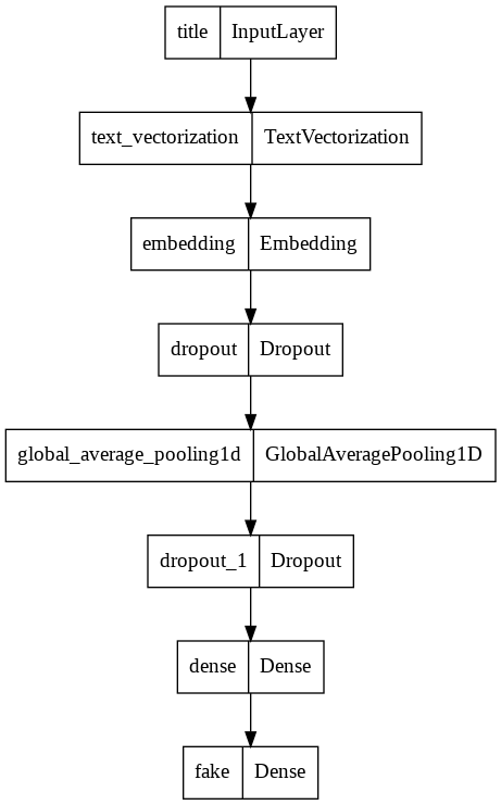
Now we’re ready to create our first model, which will only use the title to classify the article as fake or not. We’ll use the functional API to assembly our layers:

title_features = vectorize_layer(title_input) #vectorize text input
title_features = layers.Embedding(size_vocabulary, output_dim = 3, name="embedding")(title_features)
title_features = layers.Dropout(0.2)(title_features) #dropout for overfitting
title_features = layers.GlobalAveragePooling1D()(title_features)
title_features = layers.Dropout(0.2)(title_features) #dropout for overfitting
title_features = layers.Dense(32, activation='relu')(title_features)

# output layer
title_output = layers.Dense(2, name = "fake")(title_features)

Now let’s put it all together and take a look:

model1 = keras.Model(
      inputs = title_input,
      outputs = title_output
)

model1.summary()

Model: "model"
_________________________________________________________________
 Layer (type)                Output Shape              Param #   
=================================================================
 title (InputLayer)          [(None, 1)]               0         
                                                                 
 text_vectorization (TextVec  (None, 500)              0         
 torization)                                                     
                                                                 
 embedding (Embedding)       (None, 500, 3)            6000      
                                                                 
 dropout (Dropout)           (None, 500, 3)            0         
                                                                 
 global_average_pooling1d (G  (None, 3)                0         
 lobalAveragePooling1D)                                          
                                                                 
 dropout_1 (Dropout)         (None, 3)                 0         
                                                                 
 dense (Dense)               (None, 32)                128       
                                                                 
 fake (Dense)                (None, 2)                 66        
                                                                 
=================================================================
Total params: 6,194
Trainable params: 6,194
Non-trainable params: 0
_________________________________________________________________

Or if you want to visualize it:

keras.utils.plot_model(model1)

Now let’s compile it:

model1.compile(optimizer="adam",
              loss = losses.SparseCategoricalCrossentropy(from_logits=True),
              metrics=["accuracy"])

Train it:

history1 = model1.fit(train, 
                    validation_data=val,
                    epochs = 20)

Epoch 1/20


/usr/local/lib/python3.7/dist-packages/keras/engine/functional.py:559: UserWarning: Input dict contained keys ['text'] which did not match any model input. They will be ignored by the model.
  inputs = self._flatten_to_reference_inputs(inputs)


180/180 [==============================] - 5s 7ms/step - loss: 0.6924 - accuracy: 0.5181 - val_loss: 0.6911 - val_accuracy: 0.5354
Epoch 2/20
180/180 [==============================] - 1s 7ms/step - loss: 0.6902 - accuracy: 0.5247 - val_loss: 0.6867 - val_accuracy: 0.5314
Epoch 3/20
180/180 [==============================] - 1s 7ms/step - loss: 0.6729 - accuracy: 0.6078 - val_loss: 0.6432 - val_accuracy: 0.8633
Epoch 4/20
180/180 [==============================] - 1s 7ms/step - loss: 0.5800 - accuracy: 0.7944 - val_loss: 0.4979 - val_accuracy: 0.8523
Epoch 5/20
180/180 [==============================] - 1s 7ms/step - loss: 0.4315 - accuracy: 0.8739 - val_loss: 0.3557 - val_accuracy: 0.9004
Epoch 6/20
180/180 [==============================] - 1s 7ms/step - loss: 0.3383 - accuracy: 0.8834 - val_loss: 0.2889 - val_accuracy: 0.8998
Epoch 7/20
180/180 [==============================] - 1s 7ms/step - loss: 0.2960 - accuracy: 0.8879 - val_loss: 0.2411 - val_accuracy: 0.9155
Epoch 8/20
180/180 [==============================] - 1s 7ms/step - loss: 0.2703 - accuracy: 0.8991 - val_loss: 0.2238 - val_accuracy: 0.9204
Epoch 9/20
180/180 [==============================] - 1s 7ms/step - loss: 0.2506 - accuracy: 0.9027 - val_loss: 0.2052 - val_accuracy: 0.9283
Epoch 10/20
180/180 [==============================] - 1s 7ms/step - loss: 0.2393 - accuracy: 0.9071 - val_loss: 0.2045 - val_accuracy: 0.9204
Epoch 11/20
180/180 [==============================] - 1s 7ms/step - loss: 0.2327 - accuracy: 0.9094 - val_loss: 0.1969 - val_accuracy: 0.9249
Epoch 12/20
180/180 [==============================] - 1s 7ms/step - loss: 0.2245 - accuracy: 0.9117 - val_loss: 0.1900 - val_accuracy: 0.9285
Epoch 13/20
180/180 [==============================] - 1s 6ms/step - loss: 0.2156 - accuracy: 0.9158 - val_loss: 0.1765 - val_accuracy: 0.9314
Epoch 14/20
180/180 [==============================] - 1s 6ms/step - loss: 0.2068 - accuracy: 0.9194 - val_loss: 0.1763 - val_accuracy: 0.9305
Epoch 15/20
180/180 [==============================] - 1s 7ms/step - loss: 0.2068 - accuracy: 0.9204 - val_loss: 0.1746 - val_accuracy: 0.9317
Epoch 16/20
180/180 [==============================] - 1s 6ms/step - loss: 0.2017 - accuracy: 0.9216 - val_loss: 0.1695 - val_accuracy: 0.9373
Epoch 17/20
180/180 [==============================] - 1s 7ms/step - loss: 0.1976 - accuracy: 0.9241 - val_loss: 0.1615 - val_accuracy: 0.9373
Epoch 18/20
180/180 [==============================] - 1s 6ms/step - loss: 0.1939 - accuracy: 0.9244 - val_loss: 0.1612 - val_accuracy: 0.9377
Epoch 19/20
180/180 [==============================] - 1s 6ms/step - loss: 0.1898 - accuracy: 0.9256 - val_loss: 0.1594 - val_accuracy: 0.9386
Epoch 20/20
180/180 [==============================] - 1s 6ms/step - loss: 0.1911 - accuracy: 0.9265 - val_loss: 0.1492 - val_accuracy: 0.9481

So, we’re hitting mid 90’s for accuracy on our validation set just on title alone! Validation performance actually slightly exceed training performance…guess we’re not overfitting!

Second Model

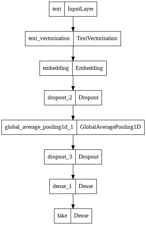
For this model we’re going to follow the same proceedure, except using only the article text rather than only the article title.

text_features = vectorize_layer(text_input) #vectorize text input
text_features = layers.Embedding(size_vocabulary, output_dim = 3, name="embedding2")(text_features)
text_features = layers.Dropout(0.2)(text_features) #dropout for overfitting
text_features = layers.GlobalAveragePooling1D()(text_features)
text_features = layers.Dropout(0.2)(text_features) #dropout for overfitting
text_features = layers.Dense(32, activation='relu')(text_features)

# output layer
text_output = layers.Dense(2, name = "fake")(text_features)

model2 = keras.Model(
      inputs = text_input,
      outputs = text_output
)

model2.summary()

Model: "model_4"
_________________________________________________________________
 Layer (type)                Output Shape              Param #   
=================================================================
 text (InputLayer)           [(None, 1)]               0         
                                                                 
 text_vectorization (TextVec  (None, 500)              0         
 torization)                                                     
                                                                 
 embedding2 (Embedding)      (None, 500, 3)            6000      
                                                                 
 dropout_4 (Dropout)         (None, 500, 3)            0         
                                                                 
 global_average_pooling1d_2   (None, 3)                0         
 (GlobalAveragePooling1D)                                        
                                                                 
 dropout_5 (Dropout)         (None, 3)                 0         
                                                                 
 dense_3 (Dense)             (None, 32)                128       
                                                                 
 fake (Dense)                (None, 2)                 66        
                                                                 
=================================================================
Total params: 6,194
Trainable params: 6,194
Non-trainable params: 0
_________________________________________________________________

keras.utils.plot_model(model2)

model2.compile(optimizer="adam",
              loss = losses.SparseCategoricalCrossentropy(from_logits=True),
              metrics=["accuracy"])

history2 = model2.fit(train, 
                    validation_data=val,
                    epochs = 20)

Epoch 1/20


/usr/local/lib/python3.7/dist-packages/keras/engine/functional.py:559: UserWarning: Input dict contained keys ['title'] which did not match any model input. They will be ignored by the model.
  inputs = self._flatten_to_reference_inputs(inputs)


180/180 [==============================] - 3s 15ms/step - loss: 0.6566 - accuracy: 0.6387 - val_loss: 0.5718 - val_accuracy: 0.8620
Epoch 2/20
180/180 [==============================] - 3s 14ms/step - loss: 0.4307 - accuracy: 0.8971 - val_loss: 0.2919 - val_accuracy: 0.9445
Epoch 3/20
180/180 [==============================] - 3s 14ms/step - loss: 0.2416 - accuracy: 0.9411 - val_loss: 0.1863 - val_accuracy: 0.9602
Epoch 4/20
180/180 [==============================] - 3s 14ms/step - loss: 0.1755 - accuracy: 0.9562 - val_loss: 0.1436 - val_accuracy: 0.9665
Epoch 5/20
180/180 [==============================] - 3s 14ms/step - loss: 0.1460 - accuracy: 0.9612 - val_loss: 0.1191 - val_accuracy: 0.9751
Epoch 6/20
180/180 [==============================] - 3s 14ms/step - loss: 0.1244 - accuracy: 0.9694 - val_loss: 0.1038 - val_accuracy: 0.9751
Epoch 7/20
180/180 [==============================] - 3s 14ms/step - loss: 0.1117 - accuracy: 0.9718 - val_loss: 0.0898 - val_accuracy: 0.9757
Epoch 8/20
180/180 [==============================] - 3s 14ms/step - loss: 0.1017 - accuracy: 0.9723 - val_loss: 0.0811 - val_accuracy: 0.9809
Epoch 9/20
180/180 [==============================] - 3s 14ms/step - loss: 0.0901 - accuracy: 0.9744 - val_loss: 0.0689 - val_accuracy: 0.9825
Epoch 10/20
180/180 [==============================] - 4s 21ms/step - loss: 0.0846 - accuracy: 0.9761 - val_loss: 0.0719 - val_accuracy: 0.9820
Epoch 11/20
180/180 [==============================] - 5s 25ms/step - loss: 0.0776 - accuracy: 0.9788 - val_loss: 0.0679 - val_accuracy: 0.9809
Epoch 12/20
180/180 [==============================] - 3s 15ms/step - loss: 0.0705 - accuracy: 0.9804 - val_loss: 0.0548 - val_accuracy: 0.9883
Epoch 13/20
180/180 [==============================] - 3s 14ms/step - loss: 0.0687 - accuracy: 0.9797 - val_loss: 0.0527 - val_accuracy: 0.9894
Epoch 14/20
180/180 [==============================] - 3s 15ms/step - loss: 0.0628 - accuracy: 0.9826 - val_loss: 0.0438 - val_accuracy: 0.9892
Epoch 15/20
180/180 [==============================] - 3s 14ms/step - loss: 0.0604 - accuracy: 0.9828 - val_loss: 0.0515 - val_accuracy: 0.9874
Epoch 16/20
180/180 [==============================] - 3s 14ms/step - loss: 0.0601 - accuracy: 0.9829 - val_loss: 0.0464 - val_accuracy: 0.9879
Epoch 17/20
180/180 [==============================] - 3s 14ms/step - loss: 0.0527 - accuracy: 0.9853 - val_loss: 0.0418 - val_accuracy: 0.9899
Epoch 18/20
180/180 [==============================] - 3s 14ms/step - loss: 0.0534 - accuracy: 0.9841 - val_loss: 0.0347 - val_accuracy: 0.9919
Epoch 19/20
180/180 [==============================] - 3s 14ms/step - loss: 0.0527 - accuracy: 0.9833 - val_loss: 0.0330 - val_accuracy: 0.9921
Epoch 20/20
180/180 [==============================] - 3s 14ms/step - loss: 0.0476 - accuracy: 0.9860 - val_loss: 0.0306 - val_accuracy: 0.9917

Wow, validation accuracy one again exceeds training accuracy, this time consistently hitting around 99%!

Third Model

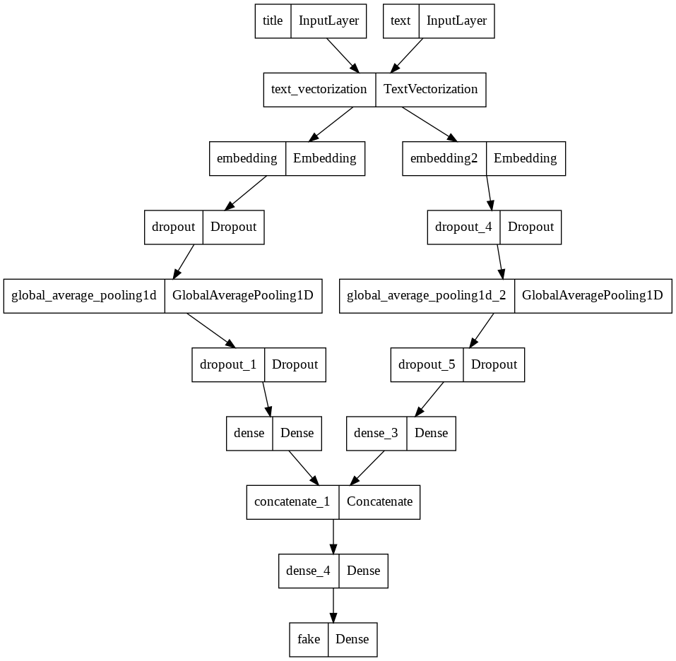
For this last model we’re going to combine both text and title and will require us to concatinate our prior two pipelines:

main = layers.concatenate([title_features, text_features], axis=1)

Then add a final dense layer:

main = layers.Dense(32, activation='relu')(main)

Finally a new output layer:

output = layers.Dense(2, name="fake")(main) 

From here, it’s the same as before:

model3 = keras.Model(
    inputs = [title_input, text_input],
    outputs = output
)

model3.summary()

Model: "model_7"
__________________________________________________________________________________________________
 Layer (type)                   Output Shape         Param #     Connected to                     
==================================================================================================
 title (InputLayer)             [(None, 1)]          0           []                               
                                                                                                  
 text (InputLayer)              [(None, 1)]          0           []                               
                                                                                                  
 text_vectorization (TextVector  (None, 500)         0           ['title[0][0]',                  
 ization)                                                         'text[0][0]']                   
                                                                                                  
 embedding (Embedding)          (None, 500, 3)       6000        ['text_vectorization[0][0]']     
                                                                                                  
 embedding2 (Embedding)         (None, 500, 3)       6000        ['text_vectorization[2][0]']     
                                                                                                  
 dropout (Dropout)              (None, 500, 3)       0           ['embedding[0][0]']              
                                                                                                  
 dropout_4 (Dropout)            (None, 500, 3)       0           ['embedding2[0][0]']             
                                                                                                  
 global_average_pooling1d (Glob  (None, 3)           0           ['dropout[0][0]']                
 alAveragePooling1D)                                                                              
                                                                                                  
 global_average_pooling1d_2 (Gl  (None, 3)           0           ['dropout_4[0][0]']              
 obalAveragePooling1D)                                                                            
                                                                                                  
 dropout_1 (Dropout)            (None, 3)            0           ['global_average_pooling1d[0][0]'
                                                                 ]                                
                                                                                                  
 dropout_5 (Dropout)            (None, 3)            0           ['global_average_pooling1d_2[0][0
                                                                 ]']                              
                                                                                                  
 dense (Dense)                  (None, 32)           128         ['dropout_1[0][0]']              
                                                                                                  
 dense_3 (Dense)                (None, 32)           128         ['dropout_5[0][0]']              
                                                                                                  
 concatenate_1 (Concatenate)    (None, 64)           0           ['dense[0][0]',                  
                                                                  'dense_3[0][0]']                
                                                                                                  
 dense_4 (Dense)                (None, 32)           2080        ['concatenate_1[0][0]']          
                                                                                                  
 fake (Dense)                   (None, 2)            66          ['dense_4[0][0]']                
                                                                                                  
==================================================================================================
Total params: 14,402
Trainable params: 14,402
Non-trainable params: 0
__________________________________________________________________________________________________

keras.utils.plot_model(model3)

model3.compile(optimizer="adam",
              loss = losses.SparseCategoricalCrossentropy(from_logits=True),
              metrics=["accuracy"])

history3 = model3.fit(train, 
                    validation_data=val,
                    epochs = 20)

Epoch 1/20
180/180 [==============================] - 4s 17ms/step - loss: 0.1411 - accuracy: 0.9852 - val_loss: 0.0182 - val_accuracy: 0.9993
Epoch 2/20
180/180 [==============================] - 3s 16ms/step - loss: 0.0196 - accuracy: 0.9964 - val_loss: 0.0079 - val_accuracy: 0.9996
Epoch 3/20
180/180 [==============================] - 3s 16ms/step - loss: 0.0131 - accuracy: 0.9966 - val_loss: 0.0046 - val_accuracy: 0.9996
Epoch 4/20
180/180 [==============================] - 3s 17ms/step - loss: 0.0118 - accuracy: 0.9967 - val_loss: 0.0059 - val_accuracy: 0.9991
Epoch 5/20
180/180 [==============================] - 3s 16ms/step - loss: 0.0095 - accuracy: 0.9974 - val_loss: 0.0052 - val_accuracy: 0.9996
Epoch 6/20
180/180 [==============================] - 3s 16ms/step - loss: 0.0104 - accuracy: 0.9969 - val_loss: 0.0044 - val_accuracy: 0.9996
Epoch 7/20
180/180 [==============================] - 3s 16ms/step - loss: 0.0110 - accuracy: 0.9967 - val_loss: 0.0054 - val_accuracy: 0.9993
Epoch 8/20
180/180 [==============================] - 3s 16ms/step - loss: 0.0095 - accuracy: 0.9972 - val_loss: 0.0031 - val_accuracy: 0.9996
Epoch 9/20
180/180 [==============================] - 3s 16ms/step - loss: 0.0070 - accuracy: 0.9978 - val_loss: 0.0019 - val_accuracy: 0.9998
Epoch 10/20
180/180 [==============================] - 3s 16ms/step - loss: 0.0086 - accuracy: 0.9972 - val_loss: 0.0019 - val_accuracy: 0.9996
Epoch 11/20
180/180 [==============================] - 3s 16ms/step - loss: 0.0094 - accuracy: 0.9972 - val_loss: 0.0076 - val_accuracy: 0.9989
Epoch 12/20
180/180 [==============================] - 3s 16ms/step - loss: 0.0075 - accuracy: 0.9980 - val_loss: 0.0042 - val_accuracy: 0.9993
Epoch 13/20
180/180 [==============================] - 3s 16ms/step - loss: 0.0085 - accuracy: 0.9972 - val_loss: 0.0030 - val_accuracy: 0.9996
Epoch 14/20
180/180 [==============================] - 3s 16ms/step - loss: 0.0084 - accuracy: 0.9970 - val_loss: 8.1322e-04 - val_accuracy: 1.0000
Epoch 15/20
180/180 [==============================] - 3s 16ms/step - loss: 0.0072 - accuracy: 0.9978 - val_loss: 0.0020 - val_accuracy: 0.9991
Epoch 16/20
180/180 [==============================] - 3s 16ms/step - loss: 0.0082 - accuracy: 0.9974 - val_loss: 8.0624e-04 - val_accuracy: 0.9998
Epoch 17/20
180/180 [==============================] - 3s 16ms/step - loss: 0.0088 - accuracy: 0.9974 - val_loss: 0.0060 - val_accuracy: 0.9989
Epoch 18/20
180/180 [==============================] - 3s 16ms/step - loss: 0.0075 - accuracy: 0.9978 - val_loss: 0.0037 - val_accuracy: 0.9996
Epoch 19/20
180/180 [==============================] - 3s 16ms/step - loss: 0.0087 - accuracy: 0.9971 - val_loss: 5.9027e-04 - val_accuracy: 1.0000
Epoch 20/20
180/180 [==============================] - 3s 16ms/step - loss: 0.0059 - accuracy: 0.9984 - val_loss: 0.0028 - val_accuracy: 0.9996

The combined model achieves nearly perfect accuracy (over 99%). It fluctates between perfect, and a very fractional percentage off perfect, fairly quickly. You could likely get away with reducing the epochs for this model. Overall, good results.

Model Evaluation

Now let’s see how our best model (the main, combined model) performs on unseen data.

First let’s read in the test data from a url:

test_url = "https://github.com/PhilChodrow/PIC16b/blob/master/datasets/fake_news_test.csv?raw=true"
test_df = pd.read_csv(test_url)
test_df

	Unnamed: 0	title	text	fake
0	420	CNN And MSNBC Destroy Trump, Black Out His Fa...	Donald Trump practically does something to cri...	1
1	14902	Exclusive: Kremlin tells companies to deliver ...	The Kremlin wants good news. The Russian lead...	0
2	322	Golden State Warriors Coach Just WRECKED Trum...	On Saturday, the man we re forced to call Pre...	1
3	16108	Putin opens monument to Stalin's victims, diss...	President Vladimir Putin inaugurated a monumen...	0
4	10304	BREAKING: DNC HACKER FIRED For Bank Fraud…Blam...	Apparently breaking the law and scamming the g...	1
...	...	...	...	...
22444	20058	U.S. will stand be steadfast ally to Britain a...	The United States will stand by Britain as it ...	0
22445	21104	Trump rebukes South Korea after North Korean b...	U.S. President Donald Trump admonished South K...	0
22446	2842	New rule requires U.S. banks to allow consumer...	U.S. banks and credit card companies could be ...	0
22447	22298	US Middle Class Still Suffering from Rockefell...	Dick Eastman The Truth HoundWhen Henry Kissin...	1
22448	333	Scaramucci TV Appearance Goes Off The Rails A...	The most infamous characters from Donald Trump...	1

22449 rows × 4 columns

Now to run it through our existing preprocessing functions:

test_ds = make_dataset(test_df)

To test it:

model3.evaluate(test_ds)

225/225 [==============================] - 5s 21ms/step - loss: 0.0446 - accuracy: 0.9900

[0.04461757093667984, 0.9899773001670837]

Great, it scored 99% accuracy on the unseen dataset.

#Embedding Visualization

Finally, let’s make an embedding visualization to examine patterns and associations in the words the model found the most useful in this classification task.

weights = model3.get_layer('embedding').get_weights()[0] # get the weights from the embedding layer
vocab = vectorize_layer.get_vocabulary()                # get the vocabulary from our data prep for later

from sklearn.decomposition import PCA
pca = PCA(n_components=2)
weights = pca.fit_transform(weights)

embedding_df = pd.DataFrame({
    'word' : vocab, 
    'x0'   : weights[:,0],
    'x1'   : weights[:,1]
})

fig = px.scatter(embedding_df, 
                 x = "x0", 
                 y = "x1", 
                 size = [2]*len(embedding_df),
                # size_max = 2,
                 hover_name = "word")

fig.show()

So, looking at the visualization based on the weights extracted from our embedding layer what can what see?

“the” is on it…which really should be a stopword…and it has a hefty weight assigned to it. So what happened? Well, NLTK stop words as returned by “stopwords.words(‘english’)” are lowercase, so by removing stop words prior to standardization we’re missing the upper case instances. I know this assignment was inherited from Dr. Chodrow so, Shruti and Harlin, I know you won’t take offense, but the assignment dictating we handle stopwords prior to standardization seems like mistake? As a result, “The [insert thing or people you don’t like here] Problem….” “The [XZY] Threat” sort of inflamatory, hyper-partisan titles are included as is…so our assignment’s directed order of operations here has a flaw, that ironically actually preserved a meaningful pattern of misinformation headline. Happy accidents, right Bob Ross?
Politician’s first names are weighted far heavier than their lastnames. Anecdotally this makes sense to me: Trump’s pejorative called his 2016 opponent “crooked Hillary,” not “crooked Hillary Clinton.” It’s easier to implicitly and sexistly diminish her by refering to her as “Hillary”—emphasizing gender—rather than by her literally presidental last name. On the flip side, the most overtly biased commentators aren’t fond of saying “President Trump”, instead going with “Donald Trump”. It sticks in their mouth much in the way “President Obama” did for sensationalist right wing writers, who instead tended to use “Barack Obama” or “Barack Hussein Obama” to emphasize the “foreigness” of his name.
“Our”, “your”, and “america” are all clustered together. Once again, makes sense, nothing says click-bait like a personal appeal: “coming for your guns,” “ruining our country,” etc. It applies ownership to a larger concept and makes the sensationalized headline a personal matter.
Things people/groups never call themselves: “is” is next to “racist”, “leftist” is next to “radical”. I’m guessing the AP (Associated Press) wire didn’t flatout lead with “[insert candidate you don’t like here] is racist” or “radical leftists are ruining [insert something you like here]”. It’s just not how actual news phrases things.
Proper nouns for international people/places aren’t very weighted. “Japan”, “Macron”, “Myanmar” aren’t fodder for misinformation the way domestic matters seem to be. Once again, makes sense: foreign affairs aren’t salient and emotionally enough to the average American to rile them up to suspend disbelief, embrace confirmation bias, and eat up misinformation. In terms of the usefulness of these words for our classification, well, for every cry of “Trump is owned by the Kremlin” or “Biden is owned by China” theres probably threefold as many articles actually addressing actual trade policy with the world’s largest export manufacturer or Russia’s ongoing military actions in Syria or Ukraine…the latter two nearing a decade old. This obviously dilutes the usefulness of these words for our purposes.

Bonus observation:

“sources” and “says” are both words misinformation tends not to contain. I guess proper quotations and attributions aren’t a staple of the genre—”the prime minister’s presss office says [stuff],” “sources close to the matter…” that sort of thing. I’m also guessing that this applies to the “sources:” list at the bottom of proper articles.

Closing Thoughts

The model performed very well, however it appears to be very temporally sensitive. It is a useful tool for extrapolation within the same cultural/news epoch as its training data. That is to say that you could manually (at least as far as the fake/not fake classifcation) build a large training set and then automate the review of a larger body of articles from roughly the same period, however, the reliance of the model on specific phrasing/terminology rather than language structure means that it would likely perform far far worse with articles from 10 years ago or 10 years from now…and that’s being optimistic about it’s valid range of applicability. As always, thank you for coming to my TED talk.

Written on May 16, 2022